CNN
Table of Contents
1. CNN
1.1. Overview
cnn 适用于图像识别是因为通过 filter 可以找到符合某种空间结构的 local pattern, 所以 cnn 工作时有依赖于一个基本假设: 数据有空间结构. 如果给一个 cnn 模型输入的图像是按像素随机 shuffle 过的图像, 则 cnn 无法工作. 类似 attention 的模型也许能处理这种不包含空间结构的数据.
1.2. Conv1D
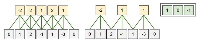
keras.layers.Conv1D(input, filters, kernel_size, strides=(1, 1), padding="valid")
- input 是三维: (batch, H, input_channel), conv 发生在 H 这一维上
- kernel_size 是一个 scaler, 与 input 的 H 对应
- stride 是一个 scaler
- 单个 filter 的尺寸是 (kernel_size, input_channel)
1.3. Conv2D
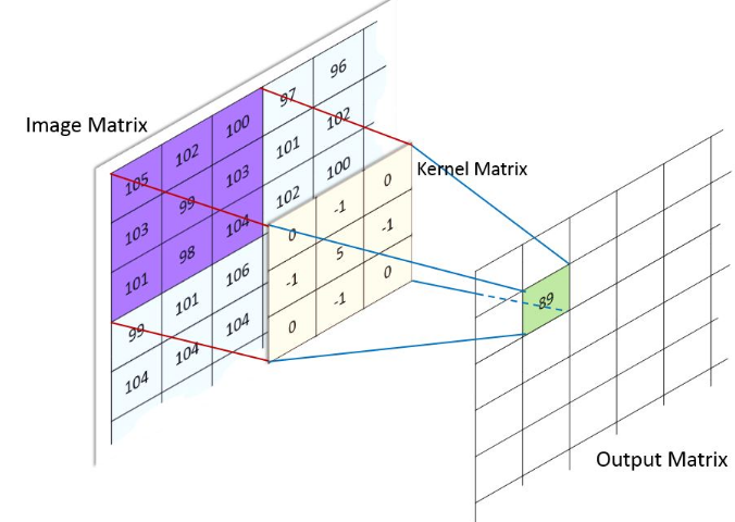
Figure 1: conv2
kernel=[0,1,2; 2,2,0; 0,1,2] 
keras.layers.Conv2D(input, filters, kernel_size, strides=(1, 1), padding="valid")
- input 是四维: (batch, H, W, input_channel), conv 发生成 H,W 这两维上
- kernel_size 是 scaler(表示 H,W 方向使用相同的值) 或 (h,w), 与 input 的 (H,W) 对应
- 单个 filter 的尺寸为 (kernel_size_h, kernel_size_w, input_channel)
1.3.1. padding
- W original size
- F kernel size
- S stride
- O output size
- P padding
\(O=\frac{W+P-F}{S}+1\)
若考虑 dilation 参数 D:
\(O=\frac{W+2*P-(D*(F-1)+1)}{S}+1\)
其中 \(D*(F-1)+1\) 相当于膨胀后的 kernel 大小
1.3.1.1. valid padding
valid padding 即 P = 0, input 中无法对齐的部分被丢弃
\(O=(W - F)//S + 1\)
1.3.1.2. same padding
same padding 时, input 中无法对齐时会在前后补 0.
选择最小的 P 使得 \(\frac{W+P-F}{S}\) 能整除.
\(O=floor(\frac{W}{S})\), 与 kernel 无关. 特别的, 当 S = 1 时, O == W, 这也是 SAME 名字的由来.
使用 same 能更容易的控制 conv 的 output shape
1.3.1.3. example
import tensorflow
import tensorflow as tf
import numpy as np
from tensorflow.keras import layers

x = np.random.normal(size=(1, 15, 1)).astype("float32")
y = layers.Conv1D(filters = 1, kernel_size = 10, strides = 3, padding = "same")(x)
y2 = layers.Conv1D(filters = 1, kernel_size = 15, strides = 3, padding = "same")(x)
y3 = layers.Conv1D(filters = 1, kernel_size = 10, strides = 3, padding = "valid")(x)
print(x.shape,y.shape,y2.shape,y3.shape)
(1, 15, 1) (1, 5, 1) (1, 5, 1) (1, 2, 1)
1.3.2. Conv2d Impl
1.3.2.1. naive
import matplotlib.pyplot as plt
import numpy as np

from skimage import io, color
import scipy.signal

def convolve2d(image, kernel):
    kernel = np.flipud(np.fliplr(kernel))
    output = np.zeros_like(image)
    # Add zero padding to the input image
    padding=kernel.shape[0]-1
    if padding%2!=0:
        print("error zero_padding")
    offset=padding//2
    image_padded = np.zeros((image.shape[0] + padding, image.shape[1] + padding))
    image_padded[offset:-offset, offset:-offset] = image
    for x in range(image.shape[1]):
        for y in range(image.shape[0]):
            output[y,x]=(kernel*image_padded[y:y+kernel.shape[0],x:x+kernel.shape[0]]).sum()
    return output

def show_result(img,title):
    global orig_image

    ax1=plt.subplot(1,2,1)
    ax1.imshow(orig_image, cmap=plt.cm.gray)
    ax1.axis("off")

    image_sharpen = img
    ax2=plt.subplot(1,2,2)
    ax2.imshow(image_sharpen, cmap=plt.cm.gray)
    ax2.axis("off")
    plt.title(title)
    plt.show()

orig_image = io.imread('../extra/image.png')
orig_image = color.rgb2gray(orig_image)
kernel_sharpen=np.array([[0,-1,0],[-1,5,-1],[0,-1,0]])
kernel_edge=np.array([[-1,-1,-1],[-1,8,-1],[-1,-1,-1]])

show_result(convolve2d(orig_image,kernel_sharpen),"sharpen")
show_result(convolve2d(orig_image,kernel_edge),"edge detection")
m=np.array([[1,1,1],[1,1,1,],[1,1,1]])
kernel=np.array([[0,1,0],[0,1,0],[0,1,0]])
print(m)
print(kernel)
print(convolve2d(m,kernel))
[[1 1 1]
 [1 1 1]
 [1 1 1]]
[[0 1 0]
 [0 1 0]
 [0 1 0]]
[[2 2 2]
 [3 3 3]
 [2 2 2]]
1.3.2.2. im2col
卷积操作实际上可以转换为普通的矩阵乘法
import numpy as np


def get_im2col_indices(x_shape, field_height, field_width, padding=1, stride=1):
  # First figure out what the size of the output should be
  N, C, H, W = x_shape
  assert (H + 2 * padding - field_height) % stride == 0
  assert (W + 2 * padding - field_height) % stride == 0
  out_height = (H + 2 * padding - field_height) // stride + 1
  out_width = (W + 2 * padding - field_width) // stride + 1

  i0 = np.repeat(np.arange(field_height), field_width)
  i0 = np.tile(i0, C)
  i1 = stride * np.repeat(np.arange(out_height), out_width)
  j0 = np.tile(np.arange(field_width), field_height * C)
  j1 = stride * np.tile(np.arange(out_width), out_height)
  i = i0.reshape(-1, 1) + i1.reshape(1, -1)
  j = j0.reshape(-1, 1) + j1.reshape(1, -1)

  k = np.repeat(np.arange(C), field_height * field_width).reshape(-1, 1)

  return (k, i, j)


def im2col_indices(x, field_height, field_width, padding=1, stride=1):
  """ An implementation of im2col based on some fancy indexing """
  # Zero-pad the input
  p = padding
  x_padded = np.pad(x, ((0, 0), (0, 0), (p, p), (p, p)), mode='constant')

  k, i, j = get_im2col_indices(x.shape, field_height, field_width, padding,
                               stride)

  cols = x_padded[:, k, i, j]
  C = x.shape[1]
  cols = cols.transpose(1, 2, 0).reshape(field_height * field_width * C, -1)
  return cols


def col2im_indices(cols, x_shape, field_height=3, field_width=3, padding=1,
                   stride=1):
  """ An implementation of col2im based on fancy indexing and np.add.at """
  N, C, H, W = x_shape
  H_padded, W_padded = H + 2 * padding, W + 2 * padding
  x_padded = np.zeros((N, C, H_padded, W_padded), dtype=cols.dtype)
  k, i, j = get_im2col_indices(x_shape, field_height, field_width, padding,
                               stride)
  cols_reshaped = cols.reshape(C * field_height * field_width, -1, N)
  cols_reshaped = cols_reshaped.transpose(2, 0, 1)
  np.add.at(x_padded, (slice(None), k, i, j), cols_reshaped)
  if padding == 0:
    return x_padded
  return x_padded[:, :, padding:-padding, padding:-padding]

pass
def convolve_im2col(image,kernel):
    image=image.reshape(1,1,160,160)
    image_col=im2col_indices(image, kernel.shape[0],kernel.shape[1])
    kernel=kernel.reshape(1,-1)
    image_conv=np.dot(kernel,image_col).reshape(160,160)
    return image_conv

show_result(convolve_im2col(orig_image,kernel_sharpen),"sharpen")
show_result(convolve_im2col(orig_image,kernel_edge),"edge")
test_image=np.arange(0,64,1).reshape(1,1,8,8)
print(test_image)
col=im2col_indices(test_image,3,3,1,1)
print(col.shape)
print(col[:,0])
print(col[:,1])
print(col[:,2])
[[[[ 0  1  2  3  4  5  6  7]
   [ 8  9 10 11 12 13 14 15]
   [16 17 18 19 20 21 22 23]
   [24 25 26 27 28 29 30 31]
   [32 33 34 35 36 37 38 39]
   [40 41 42 43 44 45 46 47]
   [48 49 50 51 52 53 54 55]
   [56 57 58 59 60 61 62 63]]]]
(9, 64)
[0 0 0 0 0 1 0 8 9]
[ 0  0  0  0  1  2  8  9 10]
[ 0  0  0  1  2  3  9 10 11]
1.3.2.3. winograd
1.4. Deconv2D
Deconv2D 有两种等价的计算方法:
Deconv2D 是一种 Upsample 的手段, 被用在大部分 Semantic Segmentation 模型中
1.4.1. 通过加 padding 和 dilation 转换为 Conv2D
1.4.2. 通过 gemm+col2im
https://bbs.cvmart.net/articles/1755 假设:
- output 的 shape 为 \(C_{out}*H_{out}*W_{out}\)
- W 的 shape 为 \(C_{out}*C_{in}*K_h*W_h\)
- input 为 \(Cin*Hin*Win\)
计算 Conv2D 的过程为:
- input 通过 im2col 转换为 \((C_{in}*K_h*K_w)*H_{out}*W_{out}\)
- \(W = C_{out}*(C_{in}*K_h*K_w) \implies output = W * input = C_{out}*H_{out}*W_{out}\)
计算 Deconv2D 的过程为:
- \(W^T = C_{out}*(K_h*W_h)*C_{in}\)
- \(output = W^T * input = C_{out}*(K_h*W_h)*H_{in}*W_{in}\)
- 通过 col2im 填充输出为 \(C_{out}*H_{out}*W_{out}\)
我觉得可以这样直观的理解一下 gemm+col2im 的方式:
conv 本质上是把长度为 k 的 block 变成一个点, 实际就是一个 matmul((x,k),(k,1))
deconv 需要把这一个点再变回长度为 k 的 block, 那么做一个 matmul((x,1),(1,k)) 就可以了…
(k,1) 是 conv kernel, (1,k) 是 deconv kernel, 所以 deconv 也叫 conv_transposed
1.5. DepthwiseConv2D
DepthwiseConv2D 最早是在 MobileNet 的应用的, 后续针对移动端的 ShuffleNet 也都会使用它, 以提高推理速度
1.5.1. DepthwiseConv2D
import numpy as np
import tensorflow as tf
from tensorflow import keras
from tensorflow.keras import layers, losses, metrics, optimizers, models


inputs = keras.Input(shape=(10, 10, 3))

outputs_ds_cnn = layers.DepthwiseConv2D(
    kernel_size=[2, 2], strides=[2, 2], padding="same"
)(inputs)
outputs_ds_cnn = layers.Conv2D(
    filters=20, kernel_size=[1, 1], strides=[1, 1], padding="same"
)(outputs_ds_cnn)
outputs_cnn = layers.Conv2D(20, kernel_size=[2, 2], strides=[2, 2], padding="same")(
    inputs
)
model_dscnn = keras.Model(inputs, outputs_ds_cnn)
model_cnn = keras.Model(inputs, outputs_cnn)

# 5,5,20
print("output_shape:")
print(outputs_ds_cnn.shape)
print(outputs_cnn.shape)
# 2,2,3,20
print("conv weight:")
print(model_cnn.layers[1].weights[0].shape)
print("ds conv weight:")
# 2,2,3,1
print(model_dscnn.layers[1].weights[0].shape)
# 1,1,3,20
print(model_dscnn.layers[2].weights[0].shape)
output_shape: (None, 5, 5, 20) (None, 5, 5, 20) conv weight: (2, 2, 3, 20) ds conv weight: (2, 2, 3, 1) (1, 1, 3, 20)
假设 input_channel 为 c, depth_multiplier 为 m.
DepthwiseConv2D 有 c 个 kernel, 每个 kernel 为 [m, 1, h, w]
input 沿 channel 划分为 c 份 , 每份为 ([N, 1, H, W]), 使用一个 kernel 做 conv2d.
一共做 c 次 conv2d, 每个 conv2d 的 output channel 为 m, 所以 DepthwiseConv2D 总的 ouput channel 为 m*c.
与 Conv2D 相比, DepthwiseConv2D 的参数个数和计算量减少很多: DepthwiseConv2D 的参数为 c 个 [m, 1, h, w], Conv2D 为 [o, c, h, w], 两者比例为 m/o
1.5.2. SeparatableConv2D
DepthwiseConv2D 后再接一个 1x1 的 Conv2D 可以把 output channel 从 m*c 变为 O
DepthwiseConv2D + 1x1 Conv2d 即 SeparatableConv2D
Backlinks
MobileNet (MobileNet): moblienet 是在 Vgg 的基础上把 3x3 conv2d 换成 SeparatableConv2D, 使得它的参数和 flops 降低很多, 更适合移动端使用.
1.5.3. group conv2d
caffe, tensorflow, pytorch 的 conv2d 均支持 group 参数, 称为 group conv2d.
group conv2d 是指 input channel/output channel 均被划分为 m 个 group, 每个 group 使用单独的 kenrel 计算 conv2d, 每个 kernel shape 为 [O/m, I/m, h, w].
例如, input channel 为 40, output channel 为 60, group 为 10, 则 kernel 为 10 个 [6, 4, h, w]
实际上, 如果像 1x1 卷积那样, 把卷积部分看做一个简单的乘法, 考虑针对 channel 的操作, 可以把 conv2d 看作 IxO 的 fc, 那么 group conv2d 就相当于 g 个 (I/g) x (O/g) 的 fc. 例如, 把 10x10 的 fc 变成两个 5x5 的 fc 再把结果拼起来.
DepthwiseConv2D 是 group conv2d 的特殊情况:
- ouput channel 等于 input channel
- group 等于 input channel
Backlinks
ShuffleNet (ShuffleNet > 1x1 group conv): 因此 shufflenet 使用 1x1 group conv2d 来降低 1x1 conv 的参数和计算量.
1.6. Dilated Conv2D
大部分的 Semantic Segmentation 模型都会使用 dilated conv2d, 用来提高 receptive field.
Backlinks
DeepLab (DeepLab): DeepLab 是 google 提出的 semantic segmentation 模型, 最新的模型是 v3 和 v3+, 主 要思想是利用多个不同 dilation rate 的 Dilated Conv2D 来融合不同尺度上的特征, 有 点类似于 Spatial Pyramid Pooling
ENet (ENet > Network > bottleneck): bottleneck 中间的 conv 变成 Dilated Conv2D
