Gradient Descent
Table of Contents
1. Gradient Descent
1.1. 梯度下降公式
梯度下降时, 先计算出 \(\nabla w=\frac{\partial{C}}{\partial{w}}\), 然后利用 \(w=w-lr*\nabla w\) 对参数进行更新. 为什么这样?
使损失函数下降
根据导数的定义: \(\Delta C \approx \nabla w*\Delta w\), 即 w 有一个 小 的增量时, \(C\) 也有一定的增量. 梯度下降的目的是给 \(w\) 一个增量, 确保 \(C\) 的增量为负数, 以便\(C\) 能下降.
若令 \(\Delta w = - \eta \nabla w\), 则 \(\Delta C \approx - \eta \nabla w * \nabla w\), 则可以确保 \(\Delta C\) 是负数
但是当 \(\eta\) 很大时无法保证 \(C\) 下降, 因为 \(\Delta C \approx \nabla w*\Delta w\) 只是在 \(\Delta w\) 较小时近似成立, 当 \(\Delta w\) 很大时, 近似条件并不满足
使损失函数收敛
随着 C 的下降, \(\nabla w\) 会越来越小, 导致 \(\Delta w\) 也越来越小趋向于 0, 从而使损失函数收敛到最小值
1.2. 等高线
import numpy as np
import matplotlib.pyplot as plt
import torch

plt.style.use("classic")
plt.subplot(121)
plt.axis('equal')
x = np.linspace(-500, 500, 1000)
y = np.linspace(-500, 500, 1000)
xx, yy = np.meshgrid(x, y)
z = xx ** 2 + yy ** 2
plt.contour(x, y, z, 20)

plt.subplot(122)
plt.axis('equal')
x = np.linspace(-500, 500, 1000)
y = np.linspace(-500, 500, 1000)
xx, yy = np.meshgrid(x, y)
z = 5 * xx ** 2 + yy ** 2
plt.contour(x, y, z, 20)

plt.show()
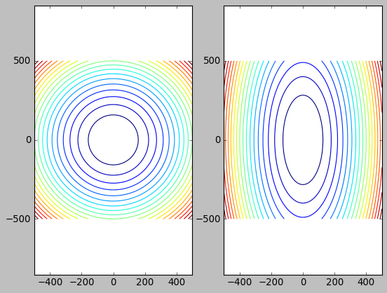
- 等高线越密, 表示越陡, 梯度的绝对值越大
可以证明梯度下降的方向与等高线的切线垂直
\(z=f(x,y)\), 按照定义, 梯度下降方向为 \([\frac{\partial{f}}{\partial{x}},\frac{\partial{f}}{\partial{y}}]\), 等高线方程为 \(f(x,y)=C\), C 为常数. 这是 y 关于 x 的隐函数, 根据隐函数求导: \(\frac{\partial{f}}{\partial{x}}+\frac{\partial{f}}{\partial{y}}*y'=0\), 可得 \(y'\) 方向为 \([-\frac{\partial{f}}{\partial{y}},\frac{\partial{f}}{\partial{x}}]\)
切线向量与梯度向量的点积: \([\frac{\partial{f}}{\partial{x}},\frac{\partial{f}}{\partial{y}}] \cdot [-\frac{\partial{f}}{\partial{y}},\frac{\partial{f}}{\partial{x}}] = 0\), 所以两者垂直
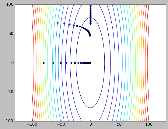
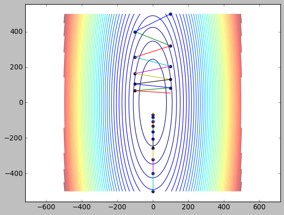
1.3. 梯度下降的速度
- 梯度下降的方向与等高线垂直
- 梯度下降的速度与梯度大小成正比, 而等高线的密度也反映了梯度的大小
所以梯度下降的速度与等高线的形状关系很大
import numpy as np
import matplotlib.pyplot as plt
import torch

alpha = 0.01

def update(x, y):
    xx = torch.tensor(x, requires_grad=True)
    yy = torch.tensor(y, requires_grad=True)
    zz = 10 * xx ** 2 + yy ** 2
    zz.backward()
    return x - alpha * xx.grad, y - alpha * yy.grad

plt.style.use("classic")
plt.axis('equal')

x = np.linspace(-100, 100, 100)
y = np.linspace(-100, 100, 100)
xx, yy = np.meshgrid(x, y)
z = 10 * xx ** 2 + yy ** 2
plt.contour(x, y, z, 20)

x, y = 0., 100.
for i in range(20):
    x, y = update(x, y)
    plt.scatter(x, y)

x, y = -70., 70.
for i in range(20):
    x, y = update(x, y)
    plt.scatter(x, y)

x, y = -100., 0.
for i in range(20):
    x, y = update(x, y)
    plt.scatter(x, y)

plt.show()
import numpy as np
import matplotlib.pyplot as plt
import torch

alpha = 0.1

def update(x, y):
    xx = torch.tensor(x, requires_grad=True)
    yy = torch.tensor(y, requires_grad=True)
    zz = 10 * xx ** 2 + yy ** 2
    zz.backward()
    return x - alpha * xx.grad, y - alpha * yy.grad

plt.axis('equal')

x = np.linspace(-500, 500, 1000)
y = np.linspace(-500, 500, 1000)
xx, yy = np.meshgrid(x, y)
z = 10 * xx ** 2 + yy ** 2
plt.contour(x, y, z, 50)

x, y = 100., 500.
for i in range(10):
    plt.scatter(x, y)
    x2, y2 = update(x, y)
    plt.plot([x, x2], [y, y2])
    x, y = x2, y2

x, y = 0., -500.
for i in range(10):
    plt.scatter(x, y)
    x2, y2 = update(x, y)
    plt.plot([x, x2], [y, y2])
    x, y = x2, y2

plt.show()
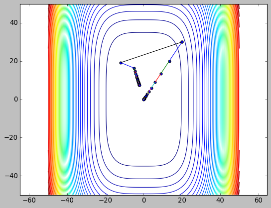
1.4. 梯度下降与 feature scaling
import numpy as np
import matplotlib.pyplot as plt
import torch

alpha = 0.02


def update_ellipse(x, y):
    xx = torch.tensor(x, requires_grad=True)
    yy = torch.tensor(y, requires_grad=True)
    zz = 20 * xx**2 + yy**2
    zz.backward()
    return x - alpha * xx.grad, y - alpha * yy.grad


def update_circle(x, y):
    xx = torch.tensor(x, requires_grad=True)
    yy = torch.tensor(y, requires_grad=True)
    zz = xx**2 + yy**2
    zz.backward()
    return x - alpha * xx.grad, y - alpha * yy.grad


EPOCH = 10

plt.style.use("classic")
plt.axis('equal')

def train():
    x = np.linspace(-100, 100, 100)
    y = np.linspace(-100, 100, 100)
    xx, yy = np.meshgrid(x, y)

    plt.subplot(121)
    z = xx**2 + yy**2
    plt.contour(xx, yy, z, 20)

    x, y = -60., 70.
    for i in range(EPOCH):
        tx, ty = x, y
        x, y = update_circle(x, y)
        plt.scatter(x, y)
        plt.plot([tx, x], [ty, y])

    plt.subplot(122)
    z = 20 * xx**2 + yy**2
    plt.contour(xx, yy, z, 20)

    x2, y2 = -60., 70.
    for i in range(EPOCH):
        tx, ty = x2, y2
        x2, y2 = update_ellipse(x2, y2)
        plt.scatter(x2, y2)
        plt.plot([tx, x2], [ty, y2])

    plt.show()
    return (x, y, x2, y2)

train()
(tensor(-39.8899), tensor(46.5383), tensor(1.00000e-06 *
-6.1440), tensor(46.5383))
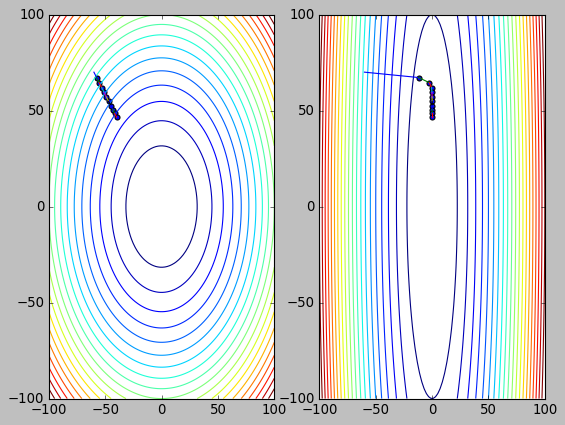
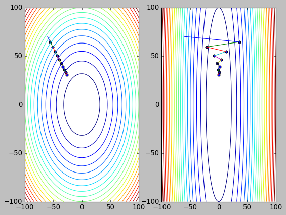
feature scaling 是通过 scaling 或 normalization 把 feature 大小调整到 [0,1] 范围内, 相当于保证等高线为圆形而非椭圆.
通过上面的代码能看到, 不论是否 scaling, 梯度下降的速度实际是相同的: 甚至未经过 scaling 的数据由于 x 方向的梯度更大反而在 x 方向下降更快. 由于两者 y 方向的梯度是相同的, 所以 y 方向会以相同的速度下降.
那么 feature scaling 的意义是什么?
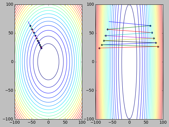
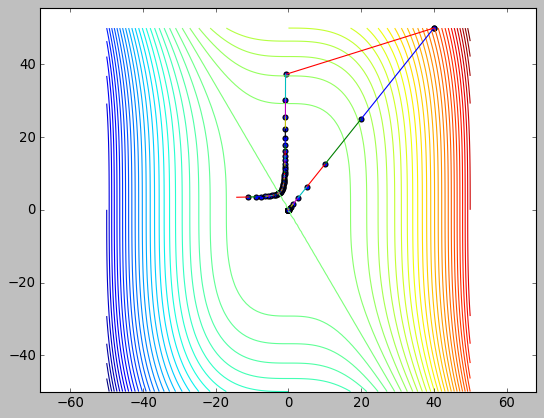
对于非 scaling 数据, 提高 learning rate 时有可能因为 zigzag 导致下降变慢甚至无法收敛, 而 scaling 后的数据一般不会有这种问题
zigzag 导致 x 方向下降变慢
alpha=0.04
train()
(tensor(-26.0633), tensor(30.4072), tensor(-0.3628), tensor(30.4072))
zigzag 导致 x 方向不收敛
alpha=0.051
train()
(tensor(-20.4604), tensor(23.8705), tensor(-88.8146), tensor(23.8705))
feature scaling 是必要的, 本质上是因为 learning rate 是需要根据梯度调整的: 梯度大时减小 learning rate, 防止 zigzag. 梯度小时增大 learning rate, 防止下降过慢. 当两个方向的梯度差别很大时, learning rate 无法兼顾.
另外, feature scaling 后, 可以使用较大的 learning rate 进行梯度下降.
1.5. 梯度下降与 batch normalization
1.6. 梯度下降与泰勒级数
泰勒级数公式: \(f(x_0+h)=f(x_0)+f'(x_0)*h+f''(x_0)*\frac{h^2}{2!}+f'''(x_0)*\frac{h^3}{3!}+\ldots\)
假设 f 的二阶以上导数很小, 只取前两项时 \(f(x_0+h)=f(x_0)+f'(x_0)*h\), 称为一阶泰勒展开, 即最开始时提到的 \(\Delta C \approx \nabla w*\Delta w\)
泰勒级数可以推广到向量1, 对于 \(f(x_0)-f(x_0+h)=-f'(x_0)*h\). \(x_0, f'(x_0), h\) 均为向量. 我们期望选一个 h (包含大小和方向), 使得 f 值下降的最大 (\(f(x_0)-f(x_0+h)\) 最大化),即\(-f'(x_0)*h\) 最大化.
若 h 方向确定, 则在保证近似相等的前提下, \(||h||\) 越大越好. 若 \(||h||\) 确定, h 方向与 \(f'(x_0)\) 相反时最好, 因为 \(f'(x_0)\cdot h=||f'(x_0)||*||h||*cos(\theta)\), \(\theta\) 为两向量夹角, \(h\) 与 \(f'(x_0)\) 夹角 180 度时, \(-f'(x_0)*h\) 最大
梯度下降忽略了泰勒级数中一阶之后的余项, 所以若 \(f''(x_0)\) 较大时, 会导致梯度下降变慢.
因为我们认为 \(x_0 \to x_0+h\) 后, \(f(x_0+h)\) 的值会下降为 \(f(x_0)+f'(x_0)*h\), 但实际值它的值仅仅下降为 \(f(x_0)+f'(x_0)*h+f''(x_0)*\frac{h^2}{2!}\)
直观的理解就是: 当二阶导数较大时, 使用一阶导数预测函数走向有较大偏差.
1.7. 牛顿法
牛顿法可以用来求 \(f(x)\) 的根:
- 首先, 对 \(f(x)\) 在 \(x_k\) 处一阶泰勒展开: \(f(x)=f(x_k)+f'(x_k)(x-x_k)\)
- \(x=x_{k+1}\) 为根时, \(f(x_{k+1})=0\), 所以 \(x_{k+1}=x_k-\frac{f(x_k)}{f'(x_k)}\)
1.8. 牛顿法与机器学习
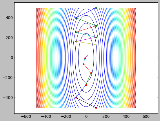
1.8.1. 牛顿法求极值
可以应用牛顿法求函数的极值, 即求 \(f'(x)\) 的根
牛顿法在求函数极值时其更新公式为: \(x_{k+1}=x_k-\frac{f'(x_k)}{f''(x_k)}\)
下面的代码中把曲线变为 \(f(x,y)=5x^3+y^3\) 来演示, 因为之前的例子中 \(f(x,y)\) 是关于 x,y 的二次函数, 二阶泰勒展开时不是近似而是完全等于原函数, 导致牛顿法只需一次迭代就会找到极值点…
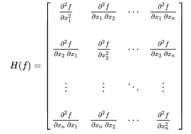
另外, 当 \(x\) 为多个变量构成的向量时, 牛顿法公式中 \(\frac{1}{f''(x_k)}\) 需要修改为 \(H(f)^{-1}\), 其中 \(H(f)\) 称为 Hessian 矩阵, 它是 \(f(x)\) 的二阶偏导组成的方阵:
import numpy as np
import matplotlib.pyplot as plt
import torch

alpha = 0.0001

def update_gd(x, y):
    xx = torch.tensor(x, requires_grad=True)
    yy = torch.tensor(y, requires_grad=True)
    zz = 10 * xx**4 + yy**4
    zz.backward()
    return x - alpha * xx.grad, y - alpha * yy.grad

def update_newton(x, y):
    # hessian 矩阵为: [120x^2,0;0,12y^2], 其逆矩阵为 [1/(120x^2),0;0;1/(12y^2)]
    # 所以 $[x,y]=[x,y]-[1/120x^2,0;0,1/12y^2]*[40x^3,4y^3]T=[x,y]-[x/3,y/]$
    x = x - x / 3.
    y = y - y / 3.
    return x, y


plt.axis('equal')

x = np.linspace(-50, 50, 100)
y = np.linspace(-50, 50, 100)
xx, yy = np.meshgrid(x, y)
z = 10 * xx**4 + yy**4
plt.contour(x, y, z, 60)

EPOCH = 20
x, y = 20., 30.
for i in range(EPOCH):
    plt.scatter(x, y)
    x2, y2 = update_newton(x, y)
    plt.plot([x, x2], [y, y2])
    x, y = x2, y2

x, y = 20., 30.
for i in range(EPOCH):
    plt.scatter(x, y)
    x2, y2 = update_gd(x, y)
    plt.plot([x, x2], [y, y2])
    x, y = x2, y2

plt.show()
1.8.2. 牛顿法的缺点
- 牛顿法计算量大, 比如求 Hessian 矩阵以及求它的逆矩阵
- 牛顿法计算的是极值, 若原函数为凸函数, 则极值就是极小值. 否则, 极值也可能是极大值或鞍点. 所以牛顿法只适用于凸函数的情形, 而机器学习中许多问题并不是凸函数, 所以无法适用牛顿法
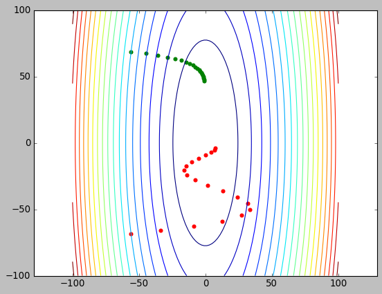
1.8.3. 举例: 牛顿法无法跳出鞍点
鞍点是既不是极小值也不是极大值的临界点, 例如 \(f(x)=x^3\) 曲线上 \(x=0\) 对应的点为鞍点.
牛顿法在 \(f(x)=x^3\) 上迭代时, 最终会稳定在 \(x=0\) 的点, 但显然这并非极小值.
理论上梯度下降也无法跳出鞍点, 因为这一点的梯度为 0, 但实际上由于 learning rate 的存在, 选择较大的 learning rate 时很容易跳过鞍点.
import numpy as np
import matplotlib.pyplot as plt
import torch

alpha = 0.0017

def update_gd(x, y):
    xx = torch.tensor(x, requires_grad=True)
    yy = torch.tensor(y, requires_grad=True)
    zz = 5 * xx**3 + yy**3
    zz.backward()
    return x - alpha * xx.grad, y - alpha * yy.grad

def update_newton(x, y):
    # hessian 矩阵为: [30x,0;0,6y], 其逆矩阵为 [1/(30x),0;0;1/(6y)]
    # 所以 $[x,y]=[x,y]-[1/30x,0;0,1/6y]*[15x^2,3y^2]T=[x,y]-[x/2,y/2]$
    x = x - x / 2.
    y = y - y / 2.
    return x, y


plt.axis('equal')

x = np.linspace(-50, 50, 100)
y = np.linspace(-50, 50, 100)
xx, yy = np.meshgrid(x, y)
z = 5 * xx**3 + yy**3
plt.contour(x, y, z, 60)

x, y = 40., 50.
for i in range(100):
    plt.scatter(x, y)
    x2, y2 = update_newton(x, y)
    plt.plot([x, x2], [y, y2])
    x, y = x2, y2

x, y = 40., 50.
for i in range(50):
    plt.scatter(x, y)
    x2, y2 = update_gd(x, y)
    plt.plot([x, x2], [y, y2])
    x, y = x2, y2

plt.show()
1.9. 牛顿法求平方根
牛顿法还有一个应用是求平方根. 两种应用的本质是一样的: 解方程的根.
对于上面求函数极值的问题, 实际上是解 \(f'(x)\) 的根. 对于求 \(K\) 的平方根的问题, 实际是解 \(f(x)=x^2-K\) 的根
以开方为例: \(x_{k+1}=x_k-\frac{f(x_k)}{f'(x_k)}=x_k-\frac{x_k^2-K}{2x_k}=\frac{x_k+\frac{K}{x_k}}{2}\),
def cube_root_newton(K):
    ret = 1
    while (abs(ret * ret * ret - K) > 1e-9):
        ret = (2 * ret + K / (ret * ret)) / 3
    return ret


def square_root_newton(K):
    ret = 1
    while (abs(ret * ret - K) > 1e-9):
        ret = (ret + K / ret) / 2
    return ret


((square_root_newton(2), square_root_newton(3), square_root_newton(4)),
 (cube_root_newton(2), cube_root_newton(3), cube_root_newton(4)))
((1.4142135623746899, 1.7320508075688772, 2.000000000000002),
(1.2599210500177698, 1.4422495703074416, 1.5874010520152708))
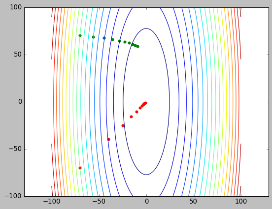
1.10. 基于 momentum 的梯度下降
momentum (动量) 是模拟的梯度下降时存在惯性: 当前梯度下降的方向不完全由当前梯度决定, 还取决于之前的方向
momentum 与梯度同向时能加快下降:
import numpy as np
import matplotlib.pyplot as plt
import torch

alpha = 0.01

vx, vy = 0, 0
def update_momentum(x, y):
    global vx, vy
    xx = torch.tensor(x, requires_grad=True)
    yy = torch.tensor(y, requires_grad=True)
    zz = 10 * xx ** 2 + yy ** 2
    zz.backward()
    # momentum
    vx = 0.8 * vx - alpha * xx.grad
    vy = 0.8 * vy - alpha * yy.grad
    return x + vx, y + vy

def update_normal(x, y):
    xx = torch.tensor(x, requires_grad=True)
    yy = torch.tensor(y, requires_grad=True)
    zz = 10 * xx ** 2 + yy ** 2
    zz.backward()
    return x - alpha * xx.grad, y - alpha * yy.grad

plt.style.use("classic")
plt.axis('equal')

x = np.linspace(-100, 100, 100)
y = np.linspace(-100, 100, 100)
xx, yy = np.meshgrid(x, y)
z = 10 * xx ** 2 + yy ** 2
plt.contour(x, y, z, 20)

x, y = -70., 70.
for i in range(20):
    x, y = update_normal(x, y)
    plt.scatter(x, y,color="green")

x, y = -70., -70.
for i in range(20):
    x, y = update_momentum(x, y)
    plt.scatter(x, y,color="red")

plt.show()
momentum 与梯度反向时能抑制震荡:
import numpy as np
import matplotlib.pyplot as plt
import torch

alpha = 0.1

vx, vy = 0, 0


def update_momentum(x, y):
    global vx, vy
    xx = torch.tensor(x, requires_grad=True)
    yy = torch.tensor(y, requires_grad=True)
    zz = 10 * xx**2 + yy**2
    zz.backward()
    # momentum
    vx = 0.5 * vx - alpha * xx.grad
    vy = 0.5 * vy - alpha * yy.grad
    return x + vx, y + vy


def update_normal(x, y):
    xx = torch.tensor(x, requires_grad=True)
    yy = torch.tensor(y, requires_grad=True)
    zz = 10 * xx**2 + yy**2
    zz.backward()
    return x - alpha * xx.grad, y - alpha * yy.grad


plt.axis('equal')

x = np.linspace(-500, 500, 1000)
y = np.linspace(-500, 500, 1000)
xx, yy = np.meshgrid(x, y)
z = 10 * xx**2 + yy**2
plt.contour(x, y, z, 50)

x, y = 100., 500.
for i in range(6):
    plt.scatter(x, y, color="green")
    x2, y2 = update_normal(x, y)
    plt.plot([x, x2], [y, y2])
    x, y = x2, y2

x, y = 100., -500.
for i in range(6):
    plt.scatter(x, y, color="red")
    x2, y2 = update_momentum(x, y)
    plt.plot([x, x2], [y, y2])
    x, y = x2, y2

plt.show()
1.11. 基于学习率调整的梯度下降
上述的方法中, 每个参数的 learning rate 都是相同的,这种做法并不合理的:对于梯度较小的特征, 应提高其学习率, 反之降低学习率 (梯度下降与 feature scaling)
类似的算法有 Adagrad, RMSprop, Adam
以 Adagrad 为例, 更新 w 的公式为:
\(w=w-\frac{\alpha}{\sqrt{\sum{dw_i^2}}}dw\), 即每个参数的学习率是原始的学习率除以当前参数类积的梯度平方和再开方. 所以, 对于梯度较小的参数, 会有较大的学习率
import numpy as np
import matplotlib.pyplot as plt
import torch

alpha = 0.01


def update_normal(x, y):
    xx = torch.tensor(x, requires_grad=True)
    yy = torch.tensor(y, requires_grad=True)
    zz = 10 * xx**2 + yy**2
    zz.backward()
    return x - alpha * xx.grad, y - alpha * yy.grad


plt.style.use("classic")
plt.axis('equal')

x = np.linspace(-100, 100, 100)
y = np.linspace(-100, 100, 100)
xx, yy = np.meshgrid(x, y)
z = 10 * xx**2 + yy**2
plt.contour(x, y, z, 20)

x, y = -70., 70.
for i in range(10):
    plt.scatter(x, y, color="green")
    x, y = update_normal(x, y)

xx = torch.tensor(-70., requires_grad=True)
yy = torch.tensor(-70., requires_grad=True)
optimizer = torch.optim.RMSprop([xx, yy], lr=3)

for i in range(10):
    plt.scatter(xx.item(), yy.item(), color="red")
    zz = 10 * xx**2 + yy**2
    optimizer.zero_grad()
    zz.backward()
    optimizer.step()
plt.show()
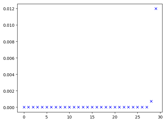
1.12. 梯度消失
把网络简化定义为:
\(\hat{y}=\underbrace{\delta_2\bigg( w_2*\overbrace{\delta_1\Big(w_1* \overbrace{\big(\delta_0(w_0*x)\big)}^\text{a0}\Big)}^\text{a1}\bigg)}_\text{a2}\)
其中 \(\delta_0\) 表示第一层的激活函数, \(w_0\) 表示第一层的权重, \(x\) 表示网络的输入, \(a_0\) 表示第一层的输出.
根据反向传播:
\(\frac{d\hat{y}}{dw_1}=\delta_2 ' * w_2 * \delta_1 ' * a_0\)
\(\frac{d\hat{y}}{dw_0}= \delta_2 ' * w_2 * \delta_1 ' * w_1 * \delta_0 ' * x\)
假设 x 和 w 已经通过 feature scaling 及权重初始化正确处理, 且使用 sigmoid 做为激活函数.
由于:
- sigmoid 最大梯度值为 sigmoid(0)=0.25
- sigmoid 的输出 a0, a1, a2 是 (0,1) 之间的数
- 权重 w0, w1, w2 通常也是小于 1 的数
因此在一次反向传播中, 权重的梯度会越来越小, \(w_0\) 的梯度会明显小于 $w_2$的梯度. 网络越深, 梯度越难以向后传递.
import numpy as np
import matplotlib.pyplot as plt
import torch

N = 1000
LAYERS = 30
plt.style.use("default")

def init_weight(in_features, out_features):
    return torch.nn.Parameter(torch.randn(in_features, out_features) / np.sqrt(in_features))


class Layer(torch.nn.Module):
    def __init__(self, in_features, out_features, n):
        super().__init__()
        self.n = n
        self.w = init_weight(in_features, out_features)
        self.bn = torch.nn.BatchNorm1d(N)

    def forward(self, input):
        ret = torch.matmul(input, self.w)
        # ret = self.bn(ret)
        ret = torch.nn.functional.sigmoid(ret)
        self.output = ret
        return ret


def visualize():
    grads = [layer.w.grad.mean().item() for layer in net]
    grads = np.array(grads)
    grads *= 100
    plt.plot(grads, "bx")
    plt.show()

criterion = torch.nn.MSELoss()

net = torch.nn.Sequential()

for i in range(LAYERS):
    net.add_module("linear%d" % (i), Layer(N, N, i + 1))

def train():
    x = torch.rand(10, N)
    loss = criterion(net(x), torch.zeros(10, N))
    loss.backward()
    visualize()

train()
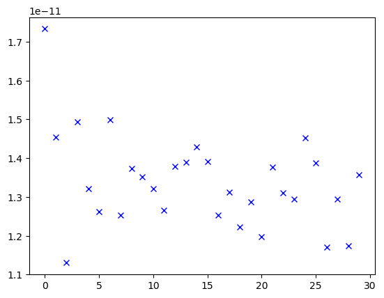
1.12.1. 如何解决
梯度消失是深度神经网络的固有问题, 一定程度上也是合理的, 它发生的原因在于激活函数: 要么激活函数的输出偏小, 要么激活函数的梯度偏小
解决方法有:
- 减少网络层数
- 为了增加激活函数的输出, 可以选择 ReLU 作为激活函数
- 为了增加激活函数的梯度, 可以选择 ReLU 或 Tanh2, 或者通过 batch normalization 调整激活函数的输入
- 修改网络的结构, 例如使用 LTSM, ResNet
import numpy as np
import matplotlib.pyplot as plt
import torch

N = 1000
LAYERS = 30
plt.style.use("default")

def init_weight(in_features, out_features):
    return torch.nn.Parameter(torch.randn(in_features, out_features) / np.sqrt(in_features))


class Layer(torch.nn.Module):
    def __init__(self, in_features, out_features, n):
        super().__init__()
        self.n = n
        self.w = init_weight(in_features, out_features)
        self.bn = torch.nn.BatchNorm1d(N)

    def forward(self, input):
        ret = torch.matmul(input, self.w)
        # ret = self.bn(ret)
        ret = torch.nn.functional.relu(ret)
        self.output = ret
        return ret


def visualize():
    grads = [layer.w.grad.mean().item() for layer in net]
    grads = np.array(grads)
    grads *= 100
    plt.plot(grads, "bx")
    plt.show()

criterion = torch.nn.MSELoss()

net = torch.nn.Sequential()

for i in range(LAYERS):
    net.add_module("linear%d" % (i), Layer(N, N, i + 1))

def train():
    x = torch.rand(10, N)
    loss = criterion(net(x), torch.zeros(10, N))
    loss.backward()
    visualize()

train()
1.13. 梯度爆炸
与梯度消失类似, 当 activation 或 dw 大于 1 时, 链式求导后会导致梯度越来越大.
解决的方法有:
- 通过 BatchNorm 限制 activation 的大小
- 通过 gradient clipping 和 gradient norm 来直接限制 gradient 的大小
1.14. sigmoid 为何需要搭配 BCELoss
BCELoss 即 binary cross entropy loss, 输出是 sigmoid 时通常使用 BCELoss.
其公式为: \(loss=-\frac{1}{n}\sum{y*log(\hat{y})}+(1-y)*log(1-\hat{y})\),
其中 \(\hat{y}=sigmoid(w^Tx+b)=\frac{1}{1+e^{-(w^T+b)}}\)
输出是 sigmoid 时为何使用 BCELoss 而不是 MSELoss?
设计一个简单的神经元: 输入为 1, 输出端采用 sigmoid 且输出为 0, 通过梯度下降学习 \(w\) 和 \(b\)
1.14.1. 使用 MSELoss
import numpy as np
import matplotlib.pyplot as plt
import torch
import torch.nn.functional as F
from tensorboardX import SummaryWriter

plt.style.use("classic")

alpha = 0.15

criterion = torch.nn.MSELoss(reduce=False)

def update_gd(x, y, step):
    xx = torch.tensor(x, requires_grad=True)
    yy = torch.tensor(y, requires_grad=True)
    zz = F.sigmoid(xx + yy)
    loss = criterion(zz, torch.tensor(0.))
    writer.add_scalar("loss", loss, step)
    loss.backward()
    return x - alpha * xx.grad, y - alpha * yy.grad

plt.axis('equal')

x = np.linspace(-10, 10, 50)
y = np.linspace(-10, 10, 50)
xx, yy = np.meshgrid(x, y)

z = F.sigmoid(torch.tensor(xx + yy).unsqueeze(0))
loss = criterion(z, torch.zeros_like(z)).squeeze(0).numpy()
CS = plt.contour(xx, yy, loss, 20)
plt.clabel(CS, inline=1, fontsize=10)

with SummaryWriter(log_dir="/tmp/runs/slooow") as writer:
    x, y = 3., 2.
    for i in range(200):
        plt.scatter(x, y)
        x2, y2 = update_gd(x, y, i)
        plt.plot([x, x2], [y, y2])
        x, y = x2, y2

with SummaryWriter(log_dir="/tmp/runs/slow") as writer:
    x, y = 2., 2.
    for i in range(200):
        plt.scatter(x, y)
        x2, y2 = update_gd(x, y, i)
        plt.plot([x, x2], [y, y2])
        x, y = x2, y2


with SummaryWriter(log_dir="/tmp/runs/fast") as writer:
    x, y = 2., 0.
    for i in range(200):
        plt.scatter(x, y)
        x2, y2 = update_gd(x, y, i)
        plt.plot([x, x2], [y, y2])
        x, y = x2, y2

plt.show()
(x, y)
(tensor(-0.2211), tensor(-2.2211))
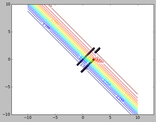

当 x 初始为 [3,2] 时, 梯度下降的很慢. 原因在于 sigmoid 函数:
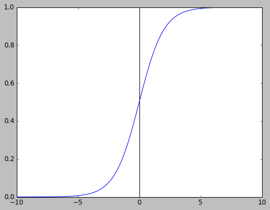
初始 x 为 [3,2], 由于 output=sigmoid(x+y), 所以对应于上图上 x=6 的点, 这一点的梯度非常小, 导致下降很慢.
根据反向传播, loss 传递到 sigmoid 时的梯度为 \(\hat{y}-y\), sigmoid 一层把梯度与它自身很小的梯度相乘后传递给 x,y, 所以最终导致 x,y 的梯度都很小.
sigmoid 的形状也反映在等高线上: 中间密两端疏.
1.14.2. 使用 BCELoss
import numpy as np
import matplotlib.pyplot as plt
import torch
import torch.nn.functional as F
from tensorboardX import SummaryWriter

plt.style.use("classic")

alpha = 0.15

criterion = torch.nn.BCELoss(reduce=False)


def update_gd(x, y, step):
    xx = torch.tensor(x, requires_grad=True)
    yy = torch.tensor(y, requires_grad=True)
    zz = F.sigmoid(xx + yy)
    loss = criterion(zz, torch.tensor(0.))
    writer.add_scalar("loss", loss, step)
    loss.backward()
    return x - alpha * xx.grad, y - alpha * yy.grad

plt.axis('equal')

x = np.linspace(-10, 10, 50)
y = np.linspace(-10, 10, 50)
xx, yy = np.meshgrid(x, y)

z = F.sigmoid(torch.tensor(xx + yy).unsqueeze(0))
loss = criterion(z, torch.zeros_like(z)).squeeze(0).numpy()
CS = plt.contour(xx, yy, loss, 20)
plt.clabel(CS, inline=1, fontsize=10)

with SummaryWriter(log_dir="/tmp/runs/bce_loss1") as writer:
    x, y = 2., 2.
    for i in range(200):
        plt.scatter(x, y)
        x2, y2 = update_gd(x, y, i)
        plt.plot([x, x2], [y, y2])
        x, y = x2, y2


with SummaryWriter(log_dir="/tmp/runs/bce_loss2") as writer:
    x, y = 2., 0.
    for i in range(200):
        plt.scatter(x, y)
        x2, y2 = update_gd(x, y, i)
        plt.plot([x, x2], [y, y2])
        x, y = x2, y2

plt.show()
(x, y)
(tensor(-1.0011), tensor(-3.0011))
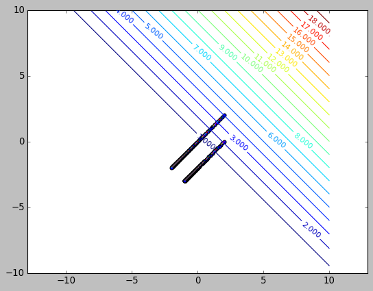
使用时 BCELoss 时, 从各个点梯度下降都很快, 而且等高线显示各处的梯度比较均匀.
\(\frac{\partial}{\partial{W}}J(W,B)=-\sum{\frac{y}{\hat{y}}}\frac{\partial}{\partial{W}}\hat{y}-\frac{1-y}{1-\hat{y}}\frac{\partial}{\partial{W}}\hat{y}\)
因此 BCELoss 反向传递到 sigmoid 时梯度为: \(\frac{1-y}{1-\hat{y}}-\frac{y}{\hat{y}}\),
当 \(\hat{y} \to 1\) 或 \(\hat{y} \to 0\) 时, 这个梯度是一个很大的值, 直观上可能抵消后面从 sigmoid 向 x,y 传递时乘上的那个极小的 sigmoid 梯度 \(\frac{\partial}{\partial{W}}\hat{y}\)
实际上把 \(\frac{\partial}{\partial{W}}\hat{y}=\hat{y}*(1-\hat{y})*x\) 代入, 最终 BCELoss 对 \(w\) 求导结果为:
\(\frac{\partial}{\partial{W}}J(W,B) = \frac{1}{m}{\sum{(\hat{y}-y})*x}\)
对比 MSELoss:
\(\frac{\partial}{\partial{W}}J(W,B) = \frac{1}{m}{\sum{(\hat{y}-y})*\hat{y}'}\)
可见 BCELoss 求导时把 sigmoid 的导数抵消了, 所以梯度会比较大.
Backlinks
Deep Learning (Deep Learning > logistic regression > cost function): logistic regression 没有使用 mse 做为 cost function sigmoid 为何需要搭配 BCELoss
