Kalman Filter
Table of Contents
1. Kalman Filter
https://www.kalmanfilter.net/CN/default_cn.aspx
https://stackoverflow.com/questions/43377626/how-to-use-kalman-filter-in-python-for-location-data
https://www.bilibili.com/video/BV1TW411N7Hg/
http://www.bzarg.com/p/how-a-kalman-filter-works-in-pictures/
1.1. Overview
- \(K_n=\frac{p_{n-1}}{p_{n-1}+r_{n}}\)
- \(p_n=(1-K_n)p_{n-1}\)
- \(\hat{x}_n=(1-K_n)\hat{x}_{n-1}+K_nZ_n\)
- \(\hat{x}_n = \hat{x}_{n-1}\)
- \(p_n = p_{n-1}\)
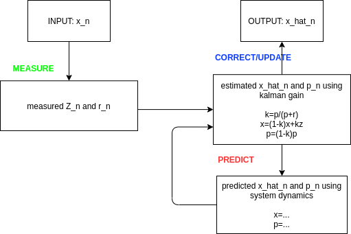
1.1.1. 初始化
kalman filter update 时需要的前一时刻的数据, 包含:
- \(p_{n-1}\) predicted variance
- \(X_{n-1}\) predicted state
1.1.2. measure
通过 measure 获得:
- \(r_n\) measured variance
- \(Z_n\) measured state
1.1.3. correct
通过 measured 来更正 predicted
- 通过公式 1 计算 \(K_n\)
- 通过公式 2 计算 \(p_n\)
- 通过公式 3 计算 \(\hat{x}_n\)
1.1.4. predict
根据系统的 dynamics 预测 x, p
若系统是 constant dynamics, 则不需要 predict, 直接 \(x_{n}=x_{n-1}\)
1.2. Example
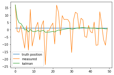
1.2.1. constant dynamics
import numpy as np
import matplotlib.pyplot as plt

t = np.arange(50)
position = np.ones(50)

STD_POSITION = 10
poisy_position = position + np.random.normal(0, STD_POSITION, size=(position.shape[0]))

plt.plot(t, position, label="truth position")
plt.plot(t, poisy_position, label="measured")

predicts = [poisy_position[0]]
position_predict = predicts[0]

p = 100
r = STD_POSITION ** 2
for i in range(1, 50):
    k = p / (p + r)
    position_predict = position_predict * (1 - k) + poisy_position[i] * k
    p = (1 - k) * p
    predicts.append(position_predict)

plt.plot(t, predicts, label="kalman")

plt.legend()
plt.show()
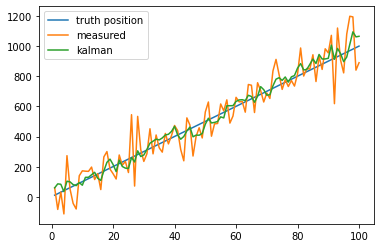
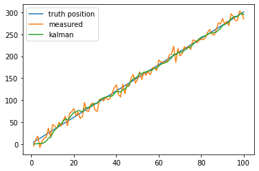
1.2.2. non-constant dynamics
import numpy as np
import matplotlib.pyplot as plt

t = np.linspace(1, 100, 100)
a = 5
position = 10 * t + 1

STD_POSITION = 100
STD_IMU = 30

poisy_position = position + np.random.normal(0, STD_POSITION, size=(t.shape[0]))

plt.plot(t, position, label="truth position")
plt.plot(t, poisy_position, label="measured")

predicts = [poisy_position[0]]
position_predict = predicts[0]

p = 0
r = STD_POSITION ** 2
for i in range(1, 100):

    # ----------measure
    dv = (position[i] - position[i - 1]) + np.random.normal(0, STD_IMU)

    # ----------predict
    # 根据 dynamics 来更新 position_predict 和 p
    position_predict = position_predict + dv
    # aX+bY 仍是正常分布, 且方差为 a^2*variance(X) + b^2*variance(Y)
    p += STD_IMU ** 2

    # ----------update
    k = p / (p + r)
    position_predict = position_predict * (1 - k) + poisy_position[i] * k
    p = (1 - k) * p
    predicts.append(position_predict)


plt.plot(t, predicts, label="kalman")

plt.legend()
plt.show()
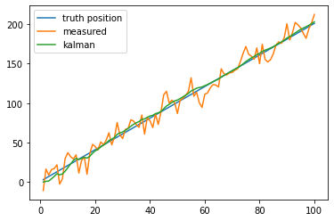
1.3. 多维 kalman filter
以一个在一维空间里匀速运动的小车为例:
- z,x 变为 2x1 矩阵 [[x],[v]]
- 需要一个 F 描述 dynamics, 设 dynamics 为: x = x+v*dt, v=v, 则 F = [[1,dt],[0,1]]
- p,r 变为 2x2 矩阵, 是一个关于 x,v 的协方差矩阵, 例如 r=[[A,0],[0,B]], 表示 x 方差为 A, v 的方差为 B. x,v 不相关, 协方差为 0
相应的五个公式变为:
https://www.kalmanfilter.net/multiSummary.html
- \(K_n=P_nH^T(HP_nH^T+R)^{-1}\)
- \(P_n=(I-K_nH)P_n(I-K_nH)^T+K_nR_n{K_n}^T\)
- \(\hat{x}_n=\hat{x}_n+K_n(Z_n-H\hat{x}_n)\)
- \(\hat{x}_{n}=F\hat{x}_{n-1}\)
- \(P_n=FP_{n}F^T+Q\)
涉及到 P, R 的公式都是 \(APA^T\) 的形式, 因为当 X, Y 是不相关的正态分布是, \(aX+bY\) 也是正态分布, 且其方差为 \(a^2\delta^2_X+b^2\delta^2_Y\)
其中 H 为 observation matrix, 用来处理 predict 中某些数据不能 measure 的情况 跟踪鼠标
import numpy as np
import matplotlib.pyplot as plt

N = 100
t = np.linspace(1, N, N)
position = 2 * t + 1

STD_POSITION = 10
STD_IMU = 3

noisy_position = position + np.random.normal(0, STD_POSITION, size=N)
noisy_speed = (position[1:] - position[:-1]) + np.random.normal(0, STD_IMU, size=N - 1)

plt.plot(t, position, label="truth position")
plt.plot(t, noisy_position, label="measured")

predicts = [0]
# 2x1
# X=[[x],[v]]
# 2x2
# F=[[1,dt],[0,1]]
# 2x2
# P=[[1,0],[0,1]]
# 2x2
# r=[[STD_POSITION**2,0],[0,STD_IMU**2]]
#
dt = 1
X = np.array([[0], [0]])
P = [[1, 0], [0, 1]]
# F,R 是我们用 kalman filter 时必需提供的两个参数, F 代表 dynamics 参数, R 代表
# correct 参数
F = np.array([[1, dt], [0, 1]])
R = [[STD_POSITION ** 2, 0], [0, STD_IMU ** 2]]

for i in range(1, N):
    # measure
    Z = [
        [noisy_position[i]],
        [(position[i] - position[i - 1]) + np.random.normal(0, STD_IMU)],
    ]
    # predict
    X = F @ X
    P = F @ P @ F.T

    # update
    K = P @ np.linalg.inv(P + R)
    X = X + K @ (Z - X)
    P = (np.eye(2) - K) @ P @ (np.eye(2) - K).T + K @ R @ K.T

    predicts.append(X[0][0])


plt.plot(t, predicts, label="kalman")

plt.legend()
plt.show()
1.4. cv2.KalmanFilter
1.4.1. 匀速运动的小车
import numpy as np
import matplotlib.pyplot as plt
import cv2

N = 100
t = np.linspace(1, N, N)
position = 3 * t + 1

STD_POSITION = 10
STD_IMU = 3

noisy_position = position + np.random.normal(0, STD_POSITION, size=N)
noisy_speed = (position[1:] - position[:-1]) + np.random.normal(0, STD_IMU, size=N - 1)

plt.plot(t, position, label="truth position")
plt.plot(t, noisy_position, label="measured")

predicts = [0]

dt = 1
F = np.array([[1, dt], [0, 1]], np.float32)
R = np.array([[STD_POSITION ** 2, 0], [0, STD_IMU ** 2]], np.float32)

filter = cv2.KalmanFilter(2, 2, 0)
# F
filter.transitionMatrix = F
# R
filter.measurementNoiseCov = R
# H
filter.measurementMatrix = np.eye(2, dtype=np.float32)
for i in range(1, N):
    # measure
    Z = np.array(
        [
            noisy_position[i],
            (position[i] - position[i - 1]) + np.random.normal(0, STD_IMU),
        ],
        np.float32,
    )
    # predict
    filter.predict()
    # corrent
    output = filter.correct(Z)
    predicts.append(output[0])

plt.plot(t, predicts, label="kalman")

plt.legend()
plt.show()
1.4.2. 跟踪鼠标
#!/usr/bin/env python3
import numpy as np
import cv2


class Stabilizer:
    """Using Kalman filter as a point stabilizer."""

    def __init__(self, state_num=4, measure_num=2, cov_process=0.0001, cov_measure=0.1):

        # Store the parameters.
        # 隐藏状态
        # X 为 [[x],[y],[v_x],[v_y]]
        self.state_num = state_num
        # 观测状态
        # Z 为 [[x],[y]]
        self.measure_num = measure_num

        # The filter itself.
        self.filter = cv2.KalmanFilter(state_num, measure_num, 0)

        # 转移矩阵: FX+Q
        # F
        self.filter.transitionMatrix = np.array(
            [[1, 0, 1, 0], [0, 1, 0, 1], [0, 0, 1, 0], [0, 0, 0, 1]], np.float32
        )
        # Q
        self.filter.processNoiseCov = np.eye(4, dtype=np.float32) * cov_process
        # 观测矩阵: HX+R
        # H, 由于 measure 信息里只有 x,y, 不包括 v_x, v_y, 所以需要用 H 把 x 中
        # 的后两个数据 mask 掉
        self.filter.measurementMatrix = np.eye(2, 4, dtype=np.float32)
        # R
        self.filter.measurementNoiseCov = np.eye(2, dtype=np.float32) * cov_measure

    def update(self, measurement):
        self.filter.predict()
        self.filter.correct(measurement)
        # statePost 是 correct 之后的 state
        # statePre 是 predict 之后, corrent 之前的 state


def main():
    global mp
    mp = np.array((2, 1), np.float32)  # measurement

    def onmouse(k, x, y, s, p):
        global mp
        mp = np.array([[np.float32(x)], [np.float32(y)]])

    cv2.namedWindow("kalman")
    cv2.setMouseCallback("kalman", onmouse)
    kalman = Stabilizer(4, 2)
    frame = np.zeros((768, 1024, 3), np.uint8)

    while True:
        kalman.update(mp)
        state = kalman.filter.statePost
        cv2.circle(frame, (int(mp[0]), int(mp[1])), 2, (255, 0, 0), -1)
        cv2.circle(frame, (int(state[0]), int(state[1])), 2, (0, 0, 255), -1)
        cv2.imshow("kalman", frame)
        k = cv2.waitKey(30) & 0xFF
        if k == 27:
            break


if __name__ == "__main__":
    main()
1.5. HMM vs. Kalman Filter
实际上,卡尔曼滤波与隐马尔可夫类似. HMM 的离散高斯动态模型, 而 kalman filter 是连续高斯动态模型. HX+R 相当于观测矩阵, FX+Q 相当于转移矩阵。卡尔曼滤波是给定观测状态序列 Z 求概率最大的隐含状态序列 X
